Markov chain Monte Carlo …
A Fisher forecast …
The cosmic distance ladder …
The dilaton …
Cosmological perturbation theory
- Baumann: Cosmology lecture notes
- Callin: How to calculate the CMB power spectrum
- Winther: Cosmology II lecture notes
Gravitational waves
Popular explanation from moving point masses and finite speed of propagation, by analogy to electromagnetic waves, water waves and sound waves.
Spontaneous symmetry breaking
Noether’s theorem
A global continuous symmetry leads to a conserved current, which in turn yields to constant charges.
Goldstone’s theorem
The spontaneous breaking of a global continuous symmetry yields massless bosons. If the symmetry is only approximate, the bosons are light.
Higgs mechanism
The spontaneous breaking of a gauge symmetry massive gauge bosons with an additional degree of freedom (instead of massless Goldstone bosons). The mass is generated by the nonzero vacuum expectation vlaue of the field in its broken phase.
Example
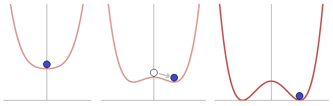
The potential of \[ \mathcal{L} = -\frac14 F_{\mu\nu} F^{\mu\nu} + (D_\mu \phi)^\dagger (D^\mu \phi) + \mu^2 (\phi^\dagger \phi) - \lambda (\phi^\dagger \phi)^2 \] with electromagnetic stress-energy tensor \(F_{\mu\nu} = \partial_\mu A_\nu - \partial_\nu A_\mu\) and covariant derivative \(D_\mu = \partial_\mu + i e A_\mu\) gets a nonzero vacuum expectation value when \(\mu^2 > 0\).
In polar coordinates \(\phi = \rho(x) e^{i \theta(x)}\): \[ \mathcal{L} = -\frac14 F_{\mu\nu} F^{\mu\nu} + (\partial_\mu \rho)^2 + \rho^2 (\partial_\mu \theta + e A_\mu)^2 + \mu^2 \rho^2 - \lambda \rho^4 \]
Noether’s theorem: global continuous symmetry → conserved currents → constant charges
Goldstone’s theorem: spontaneously broken global continuous symmetry → massless bosons (if the symmetry is approximate, the bosons are light)
Higgs mechanism: spontaneously broken gauge symmetry → massive gauge boson with additional transverse degree of freedom
Spontaneous symmetry breaking, a field develops nonzero vacuum expectation value, other fields aquire masses proportional to the nonzero vacuum expectation value. occurs whenever a charged field has a nonzero vacuum expectation value
Further reading: Noether’s Theorem, Spontaneous symmetry breaking, Goldstone boson, Higgs mechanism, Higgs boson, Gauge boson, Introduction to the physics of Higgs bosons
Exoplanets
Hawking radiation
Hawking radiation calculator for Schwarzschild black holes
N-body simulations
Shot noise
TODO
Matter evolution and growth factor
In some limit(s), matter evolves under the growth equation \[ \ddot{\delta}_m(\boldsymbol{k},t) + 2H(t) \dot{\delta}_m(\boldsymbol{k},t) - 4 \pi G \bar{\rho}_m(t) \delta_m(\boldsymbol{k},t) = 0. \] Solve this for \(\delta_m(\boldsymbol{k},t)\) and define the growth factor \(D(\boldsymbol{k},t)=\delta_m(\boldsymbol{k},t)/\delta_m(\boldsymbol{k},t_0)\) relative to today.
In a matter-dominated universe with \(\Omega_m = 1\) and \(H = H_0 \, a^{-3/2}\), the ansatz \(\delta_m(\boldsymbol{k},a) = C a^n\) gives the general analytical solution \[ \delta(\boldsymbol{k},a) = \delta_+(\boldsymbol{k},a) + \delta_m(\boldsymbol{k},a) = C_+ \, a^1 + C_- \, a^{-3/2} .\] Discarding the decaying mode \(\delta_-\), we find \(\dot{\delta}_+ = H \delta_+\). To solve the full equation, one can start in the matter-dominated era and use these analytical relations for initial conditions.
Continuity equations for perfect fluid in GR
- Continuity equation \(\nabla_\mu T^{\mu\nu} = 0\).
- Assume \(i \boldsymbol{k} \times \boldsymbol{v} \implies \boldsymbol{k} \,\|\, \boldsymbol{v} \implies \boldsymbol{k}/k = \boldsymbol{v}/v\).
- Equation of state \(\bar{P} = w \bar\rho\).
- Speed of sound \(c_s^2 = \delta P / \delta \rho\).
- If adiabatic, \(w = c_s^2\).
Background: \[ \dot{\bar\rho} = -3H(1+w)\bar\rho \]
Perturbations: \[ \dot{\delta} = 3H(w-c_s^2)\delta - (1+w) (ikva^{-1} + 3\dot\Phi)\] \[ \dot{(av)} = -ik \left( \frac{c_s^2}{w+1} \delta + \Psi\right) + 3w\dot{a}v\]
\(\sigma_8\) etc.
See book