Solving models

First create a symbolic cosmological model:

using SymBoltz
M = ΛCDM()

Creating the problem

Once the symbolic cosmological model M has been constructed, it can be turned into a numerical problem: For example:

pars = parameters_Planck18(M)
prob = CosmologyProblem(M, pars; bgjac = true, ptjac = true, bgsparse = false, ptsparse = true)

Cosmology problem for model ΛCDM
Timespan: from τ = 1.0e-6 till τ = 100.0 or a(τ) ~ 1
Stages:
  Background 1: forwards, 4 unknowns (a(τ), b₊ΔT(τ), b₊rec₊XH⁺(τ), …), dense Jacobian
  Background 2: backwards, 2 unknowns (χ(τ), b₊κ(τ)), dense Jacobian
  Perturbations: 82 unknowns (Φ(τ, k), c₊δ(τ, k), c₊θ(τ, k), …), 93.9 % sparse Jacobian
Independent parameters:
  γ₊T₀        => 2.7255
  b₊Ω₀        => 0.0493678
  h₊N         => 3.0
  c₊Ω₀        => 0.26447
  b₊YHe       => 0.2454
  h₊m_eV      => 0.02
  I₊ln_As1e10 => 3.04405
  I₊ns        => 0.965
  h           => 0.6736
  ν₊N         => 0.046

By default, analytical Jacobians are generated for both the background and perturbations. The perturbations are usually large and use sparse Jacobians for efficiency, while the background is smaller and thus faster with dense Jacobians.

SymBoltz.CosmologyProblem — Type

CosmologyProblem(
    M::System, pars::Dict, shoot_pars = Dict(), shoot_conditions = [];
    tspan = (1e-6, 100.0), terminate = M.a ~ 1,
    bg = true, pt = true, spline = true, fully_determined = true,
    bgjac = true, bgsparse = false, bgopts = (),
    ptjac = true, ptsparse = true, ptopts = (),
    debug = false, iip = true, specialize = SciMLBase.AutoSpecialize,
    kwargs...
)

Compile a numerical cosmological problem from the symbolic model M with parameters pars (mapped to numerical values). Optionally, the shooting method determines the parameters shoot_pars (mapped to initial guesses) such that the equations shoot_conditions are satisfied at the final time.

Keyword arguments

tspan: Time span over which to integrate the independent variable in M.
terminate: Terminate the first integration stage when this equation is satisfied. Shrinks the time span of later stages to the time of the termination. Pass nothing to unconditionally integrate over the entire tspan.
bg: Tuple of vectors of variables that should be integrated in each background stage. Or true to detect stages automatically from the dependency graph between variables. Variables declared with [backwards = true] are integrated backwards in time, while other variables are integrated in forward stages.
pt: Whether to compile the perturbations subproblem, if the model has $k$-dependent variables.
spline: Whether background unknowns in the perturbations are replaced by splines or integrated from scratch. Or a vector of variables that decides which (unknown/observed) variables are splined.
fully_determined: Whether the initialization system of every stage must have as many equations as unknowns.
bgjac/ptjac: Whether to generate analytical ODE Jacobians for the background/perturbation stages. Otherwise they are computed with forward-mode automatic differentiation.
bgsparse/ptsparse: Whether to use sparse or dense matrices for the ODE Jacobians in the background/perturbation stages. Larger perturbations systems with many zeros in the Jacobian are more efficient with sparse Jacobians, and smaller background systems are usually faster with dense Jacobians.
bgopts/ptopts: Extra keyword arguments passed to each ODEProblem constructor for the background/perturbation stages, overriding the options above.
debug: Whether the system of every stage is wrapped in ModelingToolkit.debug_system to help locate errors in the equations.
iip/specialize: SciMLBase type parameters forwarded to internal ODEProblem{iip, specialize}(...) constructors.
kwargs...: Extra keyword arguments passed to all ODEProblem constructors for both background/perturbation stages, overriding all options above.

source

Updating the parameters

Constructing a CosmologyProblem is an expensive operation that compiles all the symbolics down to numerics. It is not necessary to repeat this just to update parameter values. To do so, use remake to create a new problem with updated parameter values:

prob = remake(prob, [M.g.h => 0.70, M.c.Ω₀ => 0.27]) # create updated problem

Cosmology problem for model ΛCDM
Timespan: from τ = 1.0e-6 till τ = 100.0 or a(τ) ~ 1
Stages:
  Background 1: forwards, 4 unknowns (a(τ), b₊ΔT(τ), b₊rec₊XH⁺(τ), …), dense Jacobian
  Background 2: backwards, 2 unknowns (χ(τ), b₊κ(τ)), dense Jacobian
  Perturbations: 82 unknowns (Φ(τ, k), c₊δ(τ, k), c₊θ(τ, k), …), 93.9 % sparse Jacobian
Independent parameters:
  γ₊T₀        => 2.7255
  b₊Ω₀        => 0.0493678
  h₊N         => 3.0
  c₊Ω₀        => 0.27
  b₊YHe       => 0.2454
  h₊m_eV      => 0.02
  I₊ln_As1e10 => 3.04405
  I₊ns        => 0.965
  h           => 0.7
  ν₊N         => 0.046

To update the same parameters many times (e.g. in a loop), remake_function returns a function that does this more efficiently:

probf = remake_function(prob, [M.g.h, M.c.Ω₀]) # fast factory function
prob = probf([0.70, 0.27]) # create updated problem

Cosmology problem for model ΛCDM
Timespan: from τ = 1.0e-6 till τ = 100.0 or a(τ) ~ 1
Stages:
  Background 1: forwards, 4 unknowns (a(τ), b₊ΔT(τ), b₊rec₊XH⁺(τ), …), dense Jacobian
  Background 2: backwards, 2 unknowns (χ(τ), b₊κ(τ)), dense Jacobian
  Perturbations: 82 unknowns (Φ(τ, k), c₊δ(τ, k), c₊θ(τ, k), …), 93.9 % sparse Jacobian
Independent parameters:
  γ₊T₀        => 2.7255
  b₊Ω₀        => 0.0493678
  h₊N         => 3.0
  c₊Ω₀        => 0.27
  b₊YHe       => 0.2454
  h₊m_eV      => 0.02
  I₊ln_As1e10 => 3.04405
  I₊ns        => 0.965
  h           => 0.7
  ν₊N         => 0.046

SciMLBase.remake — Method

remake(prob::CosmologyProblem, pars; kwargs...)

Return a new problem with updated independent parameter values pars (a Dict, pair or vector of pairs in the form par => val). Unspecified parameters keep their values in prob.

For repeated updates, prefer remake_function instead.

Examples

newprob = remake(prob, M.c.Ω₀ => 0.3)
newprob = remake(prob, [M.c.Ω₀ => 0.3, M.g.h => 0.7])
newprob = remake(prob, Dict(M.c.Ω₀ => 0.3, M.g.h => 0.7))

source

SymBoltz.remake_function — Function

remake_function(prob::CosmologyProblem, pars; kwargs...)

Create an efficient function f for updating the values of the independent parameters pars in prob. It is called like newprob = f(vals), where vals are the new numerical values in the same order as in pars. The symbolic parameters pars can be a single parameter or a vector or tuple of parameters.

Examples

probf = remake_function(prob, M.c.Ω₀)
newprob = probf(0.3)

probf = remake_function(prob, [M.c.Ω₀, M.g.h])
newprob = probf([0.3, 0.7])

source

Solving the problem

The (updated) problem can now be solved for some wavenumbers:

ks = 10 .^ range(-2, +4, length=100)
sol = solve(prob, ks)

Cosmology solution for model ΛCDM
Stages:
  Background 1: return code Terminated; solved with Rodas5P; 746 points
  Background 2: return code Success; solved with Rodas5P; 249 points
  Perturbations (100 k-modes): return codes Success; solved with Rodas5P; 131-4641 points

CommonSolve.solve — Function

solve(
    prob::CosmologyProblem, ks::Union{Nothing, AbstractArray} = nothing;
    bgalg = default_bgalg(prob), bgreltol = 1e-7, bgabstol = 1e-7, bgopts = (),
    ptalg = default_ptalg(prob), ptreltol = 1e-5, ptabstol = 1e-5, ptopts = (),
    shootalg = default_shootalg(prob), shootabstol = 1e-5, shootopts = (),
    thread = true, verbose = false, kwargs...
)

Solve the cosmological problem prob up to the perturbative level with wavenumbers ks, or only to the background level if ks is empty or nothing.

Keyword arguments

bgalg/ptalg/shootalg: OrdinaryDiffEq and NonlinearSolve algorithms passed to the solve() of the background/perturbation/shooting problems.
bgreltol/bgabstol/ptreltol/ptabstol/shootabstol: Absolute/relative tolerances passed to the solve() of the background/perturbation/shooting problems.
bgopts/ptopts/shootopts: Extra keyword arguments passed to the solve() of the background/perturbation/shooting problems, overriding the options above.
thread: Whether multithreading is used to parallelize integration over independent perturbation $k$-modes.
verbose: Whether to print progress information while solving.
kwargs...: Extra keyword arguments passed to both background/perturbation stages, overriding all options above.

Accessing the solution

The returned solution sol can be conveniently accessed to obtain any variable y of the model M:

sol(y, τ) returns the background variable(s) $y(τ)$ as a function of conformal time(s) $τ$. It interpolates between time points using the ODE solver's custom-tailored interpolator.
sol(y, τ, k) returns the perturbation variable(s) $y(τ,k)$ as a function of the wavenumber(s) $k$ and conformal time(s) $τ$. It also interpolates linearly between the logarithms of the wavenumbers passed to solve.

Note that y can be any symbolic variables in the model M, and even expressions thereof. Unknown variables are part of the state vector integrated by the ODE solver, and are returned directly from its solution. Observed variables or expressions are functions of the unknowns, and are automatically calculated from the equations that define them in the symbolic model. For example:

τs = sol[M.τ] # get time points used in the background solution
ks = [1e0, 1e1, 1e2, 1e3] # wavenumbers
as = sol(M.g.a, τs) # scale factors
Ωms = sol((M.b.ρ + M.c.ρ) / M.G.ρ, τs) # matter-to-total density ratios
κs = sol(M.b.κ, τs) # optical depths
Φs = sol(M.g.Φ, τs, ks) # metric potentials
Φs_over_Ψs = sol(M.g.Φ / M.g.Ψ, τs, ks) # ratio between metric potentials

Plotting the solution

SymBoltz.jl includes plot recipes for easily visualizing the solution. It works similarly to the solution accessing: call plot(sol, [wavenumber(s),] x_expr, y_expr) to plot y_expr as a function of x_expr. For example, to plot some of the same quantities that we obtained above:

using Plots
p1 = plot(sol, log10(M.g.a), (M.b.ρ + M.c.ρ) / M.G.ρ)
p2 = plot(sol, log10(M.g.a), log10(abs(M.b.κ)))
p3 = plot(sol, log10(M.g.a), M.g.Φ / M.g.Ψ, ks[1:3]) # exclude last k, where Φ and Ψ cross 0
plot(p1, p2, p3, layout=(3, 1), size=(600, 800))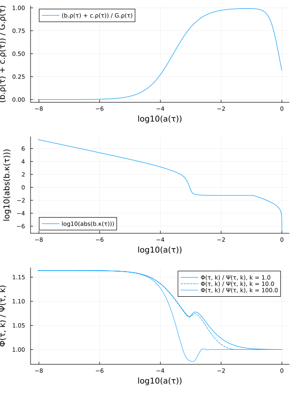

More examples are shown on the models page.

Shooting method

Some problems require tuning parameters or initial conditions to satisfy constraints at a later time. This is handled by the shooting method, which uses a rootfinder to repeatedly solve the background for different parameters to find the values that satisfies the constraints. As a trivial example, we can construct a model where the continuity equation for the cosmological constant is integrated numerically and not analytically:

g = SymBoltz.metric()
Λ = SymBoltz.cosmological_constant(g; analytical = false)
M = ΛCDM(; g, Λ)
equations(background(M.Λ))

\[ \begin{align*} \frac{\mathrm{d} ~ \rho\left( \tau \right)}{\mathrm{d}\tau} &= - 3 ~ \left( P\left( \tau \right) + \rho\left( \tau \right) \right) ~ \mathscr{H}\left( \tau \right) \\ \Omega\left( \tau \right) &= 8.3776 ~ \rho\left( \tau \right) \\ w\left( \tau \right) &= -1 \\ P\left( \tau \right) &= w\left( \tau \right) ~ \rho\left( \tau \right) \\ \mathtt{c_s^2}\left( \tau \right) &= w\left( \tau \right) \end{align*} \]

We specify to shoot for $\rho_\Lambda(\tau_\text{ini})$ and give an initial guess that is used as the starting point in Newton's method. We also specify that the constraint $H/H₀ = 1$ (in code units) must hold today:

shoot = Dict(M.Λ.ρᵢ => 0.0)
conditions = [M.g.H ~ 1]
prob = CosmologyProblem(M, pars, shoot, conditions)
sol = solve(prob; verbose = true)

Solving background 1
┌ Warning: Verbosity toggle: dt_epsilon
│  Initial timestep too small (near machine epsilon), using default: dt = 1.0e-6
└ @ OrdinaryDiffEqCore ~/.julia/packages/OrdinaryDiffEqCore/8VHiN/src/initdt.jl:222
Solving background 2
Shooting: Λ₊ρᵢ = 0.0 -> -1 + H(τ) = -0.43848443521859803
Solving background 1
Solving background 2
Solving background 1
┌ Warning: Verbosity toggle: dt_epsilon
│  Initial timestep too small (near machine epsilon), using default: dt = 1.0e-6
└ @ OrdinaryDiffEqCore ~/.julia/packages/OrdinaryDiffEqCore/8VHiN/src/initdt.jl:222
Solving background 2
Shooting: Λ₊ρᵢ = 0.05877970128512197 -> -1 + H(τ) = -0.10126121511389374
Solving background 1
Solving background 2
Solving background 1
┌ Warning: Verbosity toggle: dt_epsilon
│  Initial timestep too small (near machine epsilon), using default: dt = 1.0e-6
└ @ OrdinaryDiffEqCore ~/.julia/packages/OrdinaryDiffEqCore/8VHiN/src/initdt.jl:222
Solving background 2
Shooting: Λ₊ρᵢ = 0.08050611341447043 -> -1 + H(τ) = -0.005140126407900403
Solving background 1
Solving background 2
Solving background 1
┌ Warning: Verbosity toggle: dt_epsilon
│  Initial timestep too small (near machine epsilon), using default: dt = 1.0e-6
└ @ OrdinaryDiffEqCore ~/.julia/packages/OrdinaryDiffEqCore/8VHiN/src/initdt.jl:222
Solving background 2
Shooting: Λ₊ρᵢ = 0.08172692069040093 -> -1 + H(τ) = -1.3210486064507698e-5
Solving background 1
Solving background 2
Solving background 1
┌ Warning: Verbosity toggle: dt_epsilon
│  Initial timestep too small (near machine epsilon), using default: dt = 1.0e-6
└ @ OrdinaryDiffEqCore ~/.julia/packages/OrdinaryDiffEqCore/8VHiN/src/initdt.jl:222
Solving background 2
Shooting: Λ₊ρᵢ = 0.0817300744200061 -> -1 + H(τ) = -8.712741639271826e-11
Solving background 1
┌ Warning: Verbosity toggle: dt_epsilon
│  Initial timestep too small (near machine epsilon), using default: dt = 1.0e-6
└ @ OrdinaryDiffEqCore ~/.julia/packages/OrdinaryDiffEqCore/8VHiN/src/initdt.jl:222
Solving background 2

You can specify any number of shooting variables and conditions, but they must be equal in number to form a well-defined rootfinding problem. When there is only one shooting variable, we can also use bracketing rootfinders instead of Newton's method. To do this, replace the scalar guess with an interval:

shoot = Dict(M.Λ.ρᵢ => (0.0, 0.5))
prob = CosmologyProblem(M, pars, shoot, conditions)
sol = solve(prob; verbose = true)

Solving background 1
┌ Warning: Verbosity toggle: dt_epsilon
│  Initial timestep too small (near machine epsilon), using default: dt = 1.0e-6
└ @ OrdinaryDiffEqCore ~/.julia/packages/OrdinaryDiffEqCore/8VHiN/src/initdt.jl:222
Solving background 2
Shooting: Λ₊ρᵢ = 0.0 -> -1 + H(τ) = -0.43848443521859803
Solving background 1
┌ Warning: Verbosity toggle: dt_epsilon
│  Initial timestep too small (near machine epsilon), using default: dt = 1.0e-6
└ @ OrdinaryDiffEqCore ~/.julia/packages/OrdinaryDiffEqCore/8VHiN/src/initdt.jl:222
Solving background 2
Shooting: Λ₊ρᵢ = 0.5 -> -1 + H(τ) = 1.1222841313731222
Solving background 1
┌ Warning: Verbosity toggle: dt_epsilon
│  Initial timestep too small (near machine epsilon), using default: dt = 1.0e-6
└ @ OrdinaryDiffEqCore ~/.julia/packages/OrdinaryDiffEqCore/8VHiN/src/initdt.jl:222
Solving background 2
Shooting: Λ₊ρᵢ = 0.25 -> -1 + H(τ) = 0.5523191784826251
Solving background 1
┌ Warning: Verbosity toggle: dt_epsilon
│  Initial timestep too small (near machine epsilon), using default: dt = 1.0e-6
└ @ OrdinaryDiffEqCore ~/.julia/packages/OrdinaryDiffEqCore/8VHiN/src/initdt.jl:222
Solving background 2
Shooting: Λ₊ρᵢ = 0.11063858396231663 -> -1 + H(τ) = 0.11453280034162905
Solving background 1
┌ Warning: Verbosity toggle: dt_epsilon
│  Initial timestep too small (near machine epsilon), using default: dt = 1.0e-6
└ @ OrdinaryDiffEqCore ~/.julia/packages/OrdinaryDiffEqCore/8VHiN/src/initdt.jl:222
Solving background 2
Shooting: Λ₊ρᵢ = 0.08321590318512723 -> -1 + H(τ) = 0.0062045765053961865
Solving background 1
┌ Warning: Verbosity toggle: dt_epsilon
│  Initial timestep too small (near machine epsilon), using default: dt = 1.0e-6
└ @ OrdinaryDiffEqCore ~/.julia/packages/OrdinaryDiffEqCore/8VHiN/src/initdt.jl:222
Solving background 2
Shooting: Λ₊ρᵢ = 0.08167434556701639 -> -1 + H(τ) = -0.00023346381333078092
Solving background 1
┌ Warning: Verbosity toggle: dt_epsilon
│  Initial timestep too small (near machine epsilon), using default: dt = 1.0e-6
└ @ OrdinaryDiffEqCore ~/.julia/packages/OrdinaryDiffEqCore/8VHiN/src/initdt.jl:222
Solving background 2
Shooting: Λ₊ρᵢ = 0.08173024734802052 -> -1 + H(τ) = 7.242717834365919e-7
Solving background 1
┌ Warning: Verbosity toggle: dt_epsilon
│  Initial timestep too small (near machine epsilon), using default: dt = 1.0e-6
└ @ OrdinaryDiffEqCore ~/.julia/packages/OrdinaryDiffEqCore/8VHiN/src/initdt.jl:222
Solving background 2
Shooting: Λ₊ρᵢ = 0.08173007446098998 -> -1 + H(τ) = 8.454548172665e-11
Solving background 1
┌ Warning: Verbosity toggle: dt_epsilon
│  Initial timestep too small (near machine epsilon), using default: dt = 1.0e-6
└ @ OrdinaryDiffEqCore ~/.julia/packages/OrdinaryDiffEqCore/8VHiN/src/initdt.jl:222
Solving background 2
Shooting: Λ₊ρᵢ = 0.08173007444080624 -> -1 + H(τ) = 0.0
Solving background 1
┌ Warning: Verbosity toggle: dt_epsilon
│  Initial timestep too small (near machine epsilon), using default: dt = 1.0e-6
└ @ OrdinaryDiffEqCore ~/.julia/packages/OrdinaryDiffEqCore/8VHiN/src/initdt.jl:222
Solving background 2

Solve stages directly

For lower-level control, you can solve the background (bg) and perturbations (pt) stages separately:

SymBoltz.solvebg — Function

solvebg(bgprob::ODEProblem; alg = default_bgalg(bgprob), reltol = 1e-7, abstol = 1e-7, verbose = false, name = "Background", kwargs...)

Solve the background stage bgprob and return its solution. Its splines from previous stages must already be set, for example with setupbg.

source

solvebg(bg::Tuple; verbose = false, kwargs...)

Solve the background stages bg in order, each set up with the solutions of the previous stages (see setupbg), and return a Tuple with their solutions. If a stage fails, the later stages are not solved. Each option in kwargs can be a single value for all stages, or a Tuple with one value per stage.

source

solvebg(prob::CosmologyProblem; shootopts = (alg = default_shootalg(prob), abstol = 1e-5), verbose = false, kwargs...)

Solve all background stages of the cosmological problem prob in order, and return a Tuple with their solutions. If the problem requires shooting, all stages are solved repeatedly until the shooting conditions hold at the final time (today) of the last stage. Each option in kwargs can be a single value for all stages, or a Tuple with one value per stage.

source

SymBoltz.setupbg — Function

setupbg(bgprob::ODEProblem, bgsols::Tuple)

Prepare the background stage bgprob to be solved on top of the solutions bgsols of all previous stages: spline their unknowns into it, and integrate over the span of the last previous stage.

source

SymBoltz.solvept — Function

solvept(ptprob::ODEProblem, bgsols::Tuple, ks::AbstractArray; alg = default_ptalg(ptprob), reltol = 1e-5, abstol = 1e-5, output_func = (sol, i) -> sol, thread = true, verbose = false, kwargs...)

Solve the perturbation cosmology problem ptprob with wavenumbers ks on top of the solutions bgsols of all background stages (see solvebg). If thread and Julia is running with multiple threads, the solution of independent wavenumbers is parallellized. The return value is a vector with one ODESolution per wavenumber, or its mapping through output_func if a custom transformation is passed.

source

solvept(ptprob::ODEProblem; alg = default_ptalg(ptprob), reltol = 1e-5, abstol = 1e-5, kwargs...)

Solve the perturbation problem ptprob and return the solution. Its wavenumber and background spline must already be initialized, for example with setuppt.

Examples

# ...
prob = CosmologyProblem(M, pars)
bgsols = solvebg(prob)
ptprobf = SymBoltz.setuppt(prob.pt, bgsols)
k = 1.0
ptprob = ptprobf(k)
ptsol = solvept(ptprob)

source

Choice of ODE solver

In principle, models can be solved with any OrdinaryDiffEq.jl ODE solver. But most cosmological models have very stiff Einstein-Boltzmann equations that can only be solved by implicit solvers, while explicit solvers usually fail. For the stiff standard ΛCDM model, we find success with these solvers (from best to worst):

Rosenbrock methods: Rodas5P, Rodas4P, Rodas6P, Rodas5, Rodas4.
ESDIRK methods: KenCarp4, KenCarp47, KenCarp5, Kvaerno5, TRBDF2.
BDF methods: FBDF, QNDF.
FIRK methods: AdaptiveRadau, RadauIIA5.

See the solver benchmarks for comparisons between them.