Plotting and visualization
First, set up a cosmological problem to solve:
using SymBoltz
M = ΛCDM()
pars = parameters_Planck18(M)
prob = CosmologyProblem(M, pars)
Cosmology problem for model ΛCDM
Timespan: from τ = 1.0e-6 till τ = 100.0 or a(τ) ~ 1
Stages:
Background 1: forwards, 4 unknowns (a(τ), b₊ΔT(τ), b₊rec₊XH⁺(τ), …), dense Jacobian
Background 2: backwards, 2 unknowns (χ(τ), b₊κ(τ)), dense Jacobian
Perturbations: 82 unknowns (Φ(τ, k), c₊δ(τ, k), c₊θ(τ, k), …), 93.9 % sparse Jacobian
Independent parameters:
γ₊T₀ => 2.7255
b₊Ω₀ => 0.0493678
h₊N => 3.0
c₊Ω₀ => 0.26447
b₊YHe => 0.2454
h₊m_eV => 0.02
I₊ln_As1e10 => 3.04405
I₊ns => 0.965
h => 0.6736
ν₊N => 0.046Static plot recipes
Use SymBoltz' included plot recipes to plot the evolution of background and perturbation quantities over time:
import Plots
ks = [1e0, 1e1, 1e2, 1e3]
sol = solve(prob, ks)
p1 = Plots.plot(sol, M.χ, M.g.a)
p2 = Plots.plot(sol, log10(M.g.a), [M.g.Φ, M.g.Ψ], ks)
Plots.plot(p1, p2; layout = (2, 1), size = (600, 600))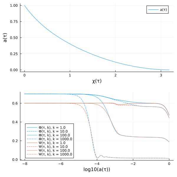
Plot the evolution of $Φ(τ,k)$ over conformal time $τ$:
ks = 10 .^ range(0, 3, length=100)
sol = solve(prob, ks)
τs = [0.0, 1e-5, 1e-4, 1e-3, 1e-2, 1e-1, 1e0]
pal = Plots.palette([:black, :orange], length(τs))
color = permutedims([pal[i] for i in eachindex(τs)])
labels = permutedims(map(τ -> "τ/H₀⁻¹ = $τ", τs))
Plots.plot(log10.(ks), permutedims(sol(M.g.Φ, τs, ks)); xlabel = "lg(k / (H₀/c))", ylabel = "Φ(τ,k)", color, labels)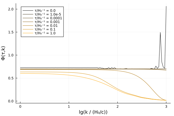
Visualize the CMB source function $S₀(τ,k)$ in a 3D plot:
ks = range(0.0, 300.0, length=100)[2:end]
sol = solve(prob, ks)
Plots.surface(sol, M.τ, M.k, M.ST; xlims = (0.03, 0.09))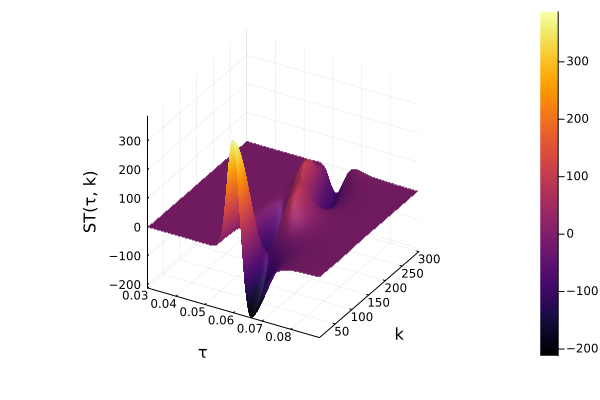
Interactive visualization
The excellent Makie plotting library can be used to interactively visualize results:
using GLMakieThe function plot_interactive builds a figure with one slider per parameter. Whenever a slider is moved, it updates the problem with the new parameter values and replots the data returned by a user-supplied function of the new problem:
obspars = [
    M.g.h => 0.60:0.01:0.70,
    M.c.Ω₀ => 0.20:0.01:0.30,
    M.b.Ω₀ => 0.02:0.01:0.10,
    M.γ.T₀ => 2.50:0.01:3.00,
    M.h.m_eV => 0.01:0.01:0.15,
    M.b.YHe => 0.20:0.01:0.30,
    M.ν.N => 2.90:0.01:3.10
]
fig = plot_interactive(prob, obspars; xlabel = "lg(a)", ylabel = "Xₑ") do prob′
    sol = solve(prob′)
    τ = SymBoltz.timeseries(sol)
    collect(zip(log10.(sol(M.g.a, τ)), sol(M.b.Xe, τ))) # [(x1, y1), (x2, y2), ...]
end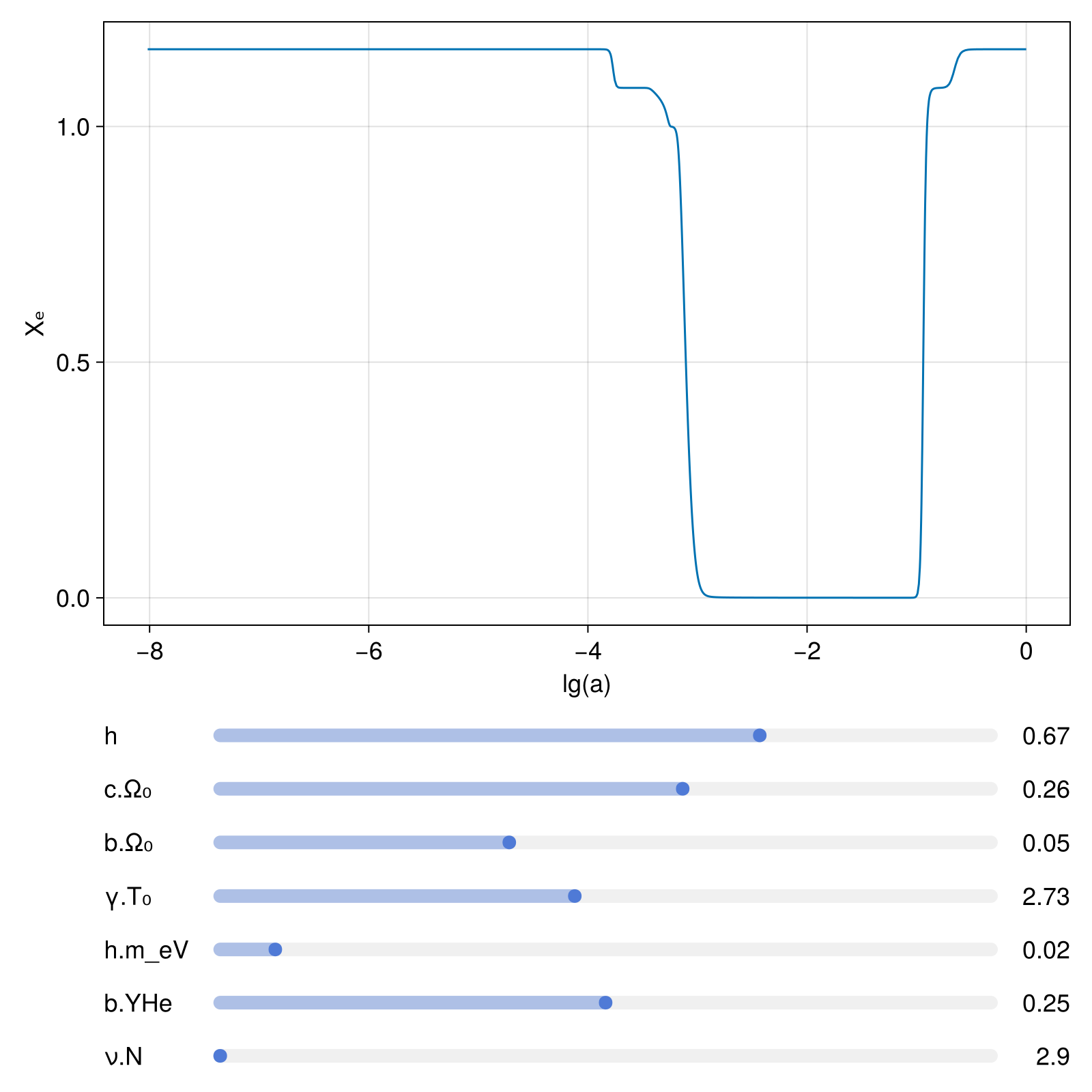
This plot is static due to limitations in the documentation building system. It is interactive when you execute the code locally.
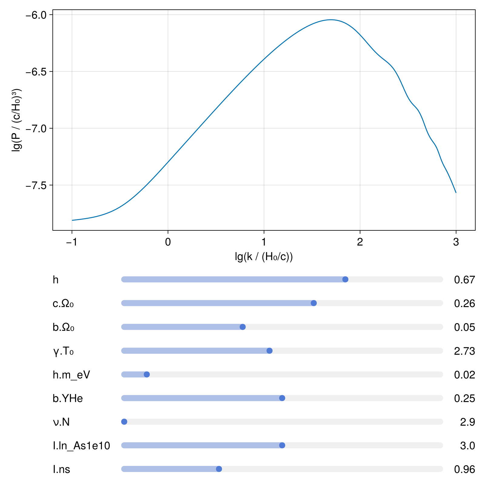
We can make a similar plot for the matter power spectrum $P(k; θ)$ as a function of cosmological parameters:
using DataInterpolations # for smoothing
obspars = [
    obspars; # extend vector from above
    M.I.ln_As1e10 => 2.0:0.1:4.0
    M.I.ns => 0.90:0.01:1.10
]
fig = plot_interactive(prob, obspars; xlabel = "lg(k / (H₀/c))", ylabel = "lg(P / (c/H₀)³)") do prob′
    lgks = unique([-1:0.5:0; 0:0.2:1; 1:0.05:3]) # as few points as possible
    ks = 10 .^ lgks
    Ps = spectrum_matter(prob′, ks; ptalg = SymBoltz.TRBDF2(), ptreltol = 1e-4, ptabstol = 1e-4)
    lgPs = log10.(Ps)

    # smoothen with spline and sample more densely
    lgPspline = CubicSpline(lgPs, lgks)
    lgks = range(lgks[begin], lgks[end]; step = 0.01)
    lgPs = lgPspline(lgks)

    collect(zip(lgks, lgPs)) # [(x1, y1), (x2, y2), ...]
end