Cosmologies (full models)
Free radiation, matter and cosmological constant (RMΛ)
SymBoltz.RMΛ — Function
RMΛ(;
    acceleration = false,
    adiabatic = true,
    g = metric(),
    r = radiation(g; adiabatic),
    m = matter(g; adiabatic),
    Λ = cosmological_constant(g; adiabatic),
    K = nothing,
    G = general_relativity(g; acceleration),
    I = harrison_zeldovich(g; name = :I),
    name = :RMΛ, kwargs...
)
Create a simple model with pure non-interacting radiation, matter and cosmological constant.
using SymBoltz, Plots
M = RMΛ()
pars = Dict(M.r.Ω₀ => 5e-5, M.m.Ω₀ => 0.3, M.g.h => 1.0, M.r.T₀ => NaN) # TODO: don't pass h and T₀ to avoid infinite loop
prob = CosmologyProblem(M, pars)
ks = [1e0, 1e1, 1e2, 1e3]
sol = solve(prob, ks)
p1 = plot(sol, log10(M.g.a), [M.r.ρ, M.m.ρ, M.Λ.ρ, M.G.ρ] ./ M.G.ρ)
p2 = plot(sol, log10(M.g.a), M.g.Φ, ks)
plot(p1, p2, layout = (2, 1), size = (600, 600))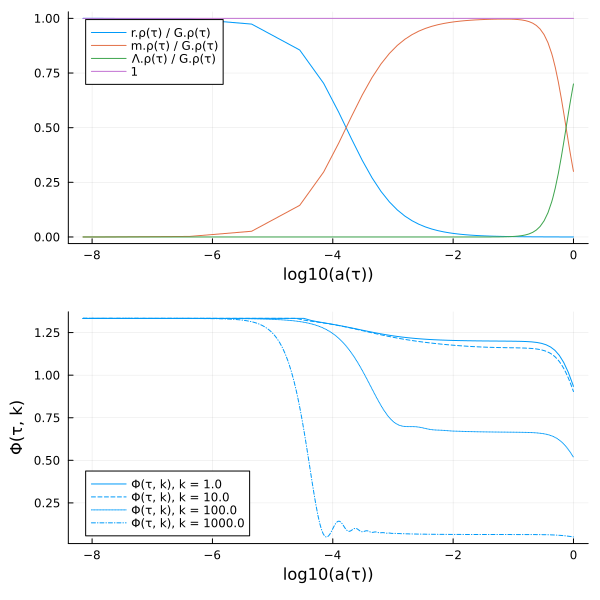
Standard ΛCDM
SymBoltz.ΛCDM — Function
ΛCDM(;
    lmax = 10,
    recombination = true,
    reionization = true,
    Hswitch = 1,
    Heswitch = 6,
    acceleration = false,
    g = metric(),
    G = general_relativity(g; acceleration),
    γ = photons(g; lmax),
    ν = massless_neutrinos(g; lmax),
    h = massive_neutrinos(g; lmax),
    c = cold_dark_matter(g; name = :c),
    b = baryons(g; recombination, reionization, Hswitch, Heswitch, name = :b),
    K = nothing,
    Λ = cosmological_constant(g),
    I = harrison_zeldovich(g; name = :I),
    matter_species = [:c, :b, :h],
    radiation_species = [:γ, :ν, :h],
    name = :ΛCDM,
    kwargs...
)
Create a ΛCDM model.
using SymBoltz, Plots
M = ΛCDM()
pars = parameters_Planck18(M)
prob = CosmologyProblem(M, pars)
ks = [1e0, 1e1, 1e2, 1e3]
sol = solve(prob, ks)
p1 = plot(sol, log10(M.g.a), [M.γ.ρ, M.ν.ρ, M.h.ρ, M.b.ρ, M.c.ρ, M.Λ.ρ, M.G.ρ] ./ M.G.ρ)
p2 = plot(sol, log10(M.g.a), M.g.Φ, ks)
plot(p1, p2, layout = (2, 1), size = (600, 600))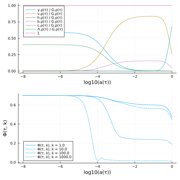
w₀wₐCDM (CPL parametrization)
SymBoltz.w0waCDM — Function
w0waCDM(; name = :w0waCDM, kwargs...)Create a ΛCDM model, but with w₀wₐ-parametrized dark energy instead of the cosmological constant.
using SymBoltz, Plots
M = w0waCDM()
pars = merge(parameters_Planck18(M), Dict(
    M.X.w0 => -0.9,
    M.X.wa => 0.2,
    M.X.cₛ² => 1.0
))
ks = [1e0, 1e1, 1e2, 1e3]
prob = CosmologyProblem(M, pars)
sol = solve(prob, ks)
p1 = plot(sol, log10(M.g.a), M.X.w)
p2 = plot(sol, log10(M.g.a), M.X.δ, ks)
plot(p1, p2, layout = (2, 1), size = (600, 600))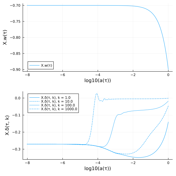
Brans-Dicke ΛCDM
SymBoltz.BDΛCDM — Function
BDΛCDM(; name = :BDΛCDM, kwargs...)Create a ΛCDM model, but with the Brans-Dicke theory of gravity instead of General Relativity.
Solve background such that H = G = 1 today, and plot scalar field and Hubble function:
using SymBoltz, Plots
M = BDΛCDM()
ks = [1e0, 1e1, 1e2, 1e3]
pars = merge(parameters_Planck18(M), Dict(M.G.ω => 100.0, M.G.ϕ̇ini => 0.0)) # unspecified: M.Λ.Ω₀, M.G.ϕini
prob = CosmologyProblem(M, pars, Dict(M.G.ϕini => 0.95, M.Λ.Ω₀ => 0.5), [M.g.ℋ ~ 1, M.G.G ~ 1])
sol = solve(prob, ks; verbose = true)
p1 = plot(sol, log10(M.g.a), [M.g.ℋ, M.G.G], ylims = (0.8, 1.2))
p2 = plot(sol, log10(M.g.a), M.G.δϕ, ks)
plot(p1, p2, layout = (2, 1), size = (600, 600))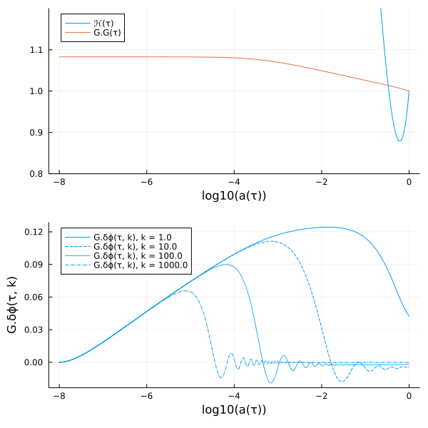
Brans-Dicke RMΛ
using SymBoltz, Plots
M = SymBoltz.BDRMΛ()
pars = Dict(M.r.Ω₀ => 5e-5, M.m.Ω₀ => 0.3, M.g.h => 1.0, M.r.T₀ => 0.0, M.G.ω => 10.0, M.G.ϕ̇ini => 0.0) # unspecified: M.Λ.Ω₀, M.G.ϕini
prob = CosmologyProblem(M, pars, Dict(M.G.ϕini => 0.8, M.Λ.Ω₀ => 0.8), [M.g.ℋ ~ 1, M.G.G ~ 1])
k = 1e3
sol = solve(prob, k; verbose = true)
p1 = plot(sol, log10(M.g.a), M.G.G)
p2 = plot(sol, log10(M.g.a), M.G.δϕ, k)
plot(p1, p2, layout = (2, 1))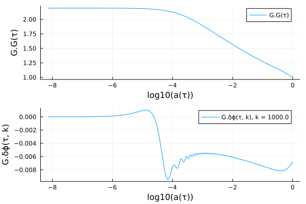
Quintessence-CDM
SymBoltz.QCDM — Function
QCDM(V; name = :QCDM, kwargs...)Create a ΛCDM model, but with the quintessence scalar field in the potential V(ϕ) as dark energy instead of the cosmological constant. One parameter must be shot for to give the dark energy density today (see quintessence).
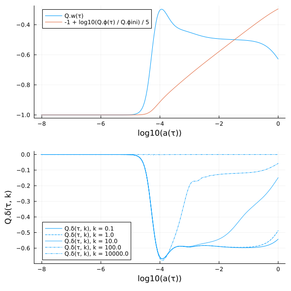
Solve a tracking quintessence field in an inverse power-law potential $V(ϕ) = V_0 (\sqrt{8π} ϕ)^{-α}$ with $α > 0$. The field starts frozen and joins the tracker solution with $w = -2/(α+2)$ during matter domination, before it accelerates the late-time expansion. The shooting method is used to determine the potential amplitude V0 such that the constraint $ℋ = 1$ holds today.
using SymBoltz, Plots
@parameters V0 α
V = ϕ -> V0 * (√(8π) * ϕ)^(-α)
M = QCDM(V)
pars = merge(parameters_Planck18(M), Dict(M.Q.α => 2.0, M.Q.ϕini => 1e-4))
prob = CosmologyProblem(M, pars, Dict(M.Q.V0 => 0.2)) # shoot V0 from initial guess
ks = [1e-1, 1e0, 1e1, 1e2, 1e4]
sol = solve(prob, ks)
p1 = plot(sol, log10(M.g.a), [M.Q.w, log10(M.Q.ϕ/M.Q.ϕini)/5 - 1])
p2 = plot(sol, log10(M.g.a), M.Q.δ, ks)
plot(p1, p2, layout = (2, 1), size = (600, 600))