Observable quantities
This page shows observable quantities that can be derived from solutions of the Einstein-Boltzmann system, such as power spectra and distances.
Primordial power spectra
SymBoltz.spectrum_primordial — Function
spectrum_primordial(k, h, As, ns=1.0; kp = 0.05*(L100/h))Compute the primordial power spectrum
\[P₀(k) = 2π² Aₛ (k/kₚ)^{nₛ-1} / k³\]
with spectral amplitude As, spectral index ns and pivot scale wavenumber kp at the wavenumber(s) k. All wavenumbers are in units of $H₀/c$, and the default pivot scale is 0.05/Mpc.
Example
using SymBoltz, Plots
M = ΛCDM()
pars = Dict(M.g.h => 0.7, M.I.As => 2e-9, M.I.ns => 0.95)
ks = 10 .^ range(-2, +4, length=100)
Ps = spectrum_primordial(ks, M, pars)
plot(log10.(ks), log10.(Ps); xlabel = "log10(k / (H₀/c))", ylabel = "log10(P / (c/H₀)³)")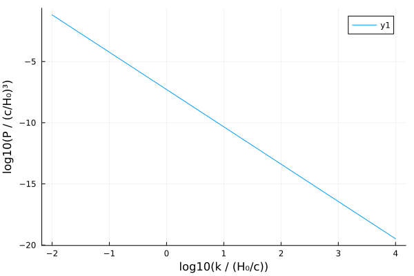
Matter power spectra
SymBoltz.spectrum_matter — Function
spectrum_matter([modes,] prob::CosmologyProblem, k[, τ]; kwargs...)Compute the matter power spectrum
\[P(τ,k) = P₀(k) |Δ(τ,k)|²\]
of the total gauge-invariant overdensity
\[Δ = (∑ₛρₛΔₛ) / (∑ₛρₛ)\]
for one or more modes at wavenumbers k and conformal time(s) τ from the problem prob. The problem is solved for the given $k$, and the matter power spectrum is saved at the given $τ$.
modesmust be:c(CDM),:b(baryons),:h(massive neutrinos),:m(matter; equivalent to $c+b+h$), a vector thereof, or unspecified to use:m.kmust be a vector of wavenumbers in units of $H₀/c$.τmust be a single or a vector of conformal times, or unspecified to use $τ = τ₀$ today.kwargs...are keyword arguments that are forwarded tosolve(prob, k; kwargs...).
spectrum_matter([modes,] sol::CosmologySolution, k[, τ]; kwargs...)Compute the matter power spectrum in the same way, but interpolate between wavenumbers and times already stored in the solution sol.
SymBoltz.spectrum_matter_nonlinear — Function
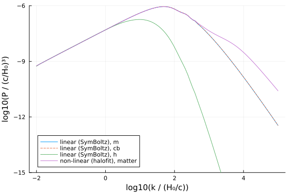
spectrum_matter_nonlinear(sol::CosmologySolution, k)Compute the nonlinear matter power spectrum from the cosmology solution sol at wavenumber(s) k using halofit implemented in MatterPower.jl.
Example
With explicitly chosen wavenumbers:
using SymBoltz, Plots
M = ΛCDM()
pars = parameters_Planck18(M)
prob = CosmologyProblem(M, pars)
ks = 10 .^ range(-2, +5, length=100)
sol = solve(prob, ks)

# Linear power spectrum
modes = [:m, :cb, :h]
Ps = spectrum_matter(modes, sol, ks)
plot(
    log10.(ks), transpose(log10.(Ps));
    xlabel = "log10(k / (H₀/c))", ylabel = "log10(P / (c/H₀)³)",
    label = permutedims("linear (SymBoltz), " .* string.(modes)), ylims = (-15, -6),
    linestyle = [:solid :dash :dot :dashdot :dashdotdot], legend_position = :bottomleft
)

# Nonlinear power spectrum (from halofit)
Ps = spectrum_matter_nonlinear(sol, ks)
plot!(
    log10.(ks), log10.(Ps);
    label = "non-linear (halofit), matter", legend_position = :bottomleft
)
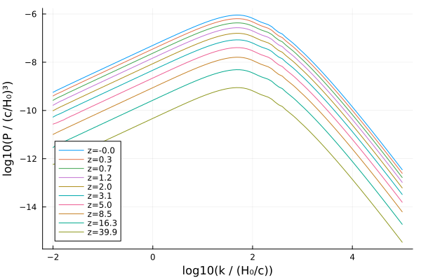
As a function of conformal time and redshift:
τs = range(sol[M.τ][end], 0.5, length=10)
Ps = spectrum_matter(sol, ks, τs)
zs = sol(M.g.z, τs) # corresponding redshifts
plot(
    log10.(ks), transpose(log10.(Ps));
    xlabel = "log10(k / (H₀/c))", ylabel = "log10(P / (c/H₀)³)",
    label = permutedims("z=".*string.(round.(zs;digits=1))),
    legend_position = :bottomleft
)
CMB power spectra
SymBoltz.spectrum_cmb — Function
spectrum_cmb(ΘlAs::AbstractMatrix, ΘlBs::AbstractMatrix, P0s::AbstractVector, ls::AbstractVector, ks::AbstractVector, ws::AbstractVector; normalization = :Cl, thread = true)Compute the angular power spectrum
\[Cₗᴬᴮ = (2/π) ∫\mathrm{d}k \, k² P₀(k) Θₗᴬ(τ₀,k) Θₗᴮ(τ₀,k)\]
for the given ls, using the quadrature weights ws for the wavenumbers ks. If normalization == :Dl, compute $Dₗ = Cₗ l (l+1) / 2π$ instead.
spectrum_cmb(modes::AbstractVector{<:Symbol}, prob::CosmologyProblem, jl::SphericalBesselCache; normalization = :Cl, kinterp = nothing, τquad = nothing, kquad = nothing, l_limber = 11, bgalg = default_bgalg(prob), bgreltol = 1e-7, bgabstol = 1e-7, bgopts = (), ptalg = default_ptalg(prob), ptreltol = 1e-5, ptabstol = 1e-5, ptopts = (), thread = true, verbose = false, kwargs...)Compute angular CMB power spectra $Cₗᴬᴮ$ at angular wavenumbers ls from the cosmological problem prob. The requested modes are specified as a vector of symbols in the form :AB, where A and B are T (temperature), E (E-mode polarization) or ψ (lensing). The spectra are of dimensionless temperature fluctuations relative to the present photon temperature $T_{γ0}$; multiply by $T_{γ0}^2$ to get dimensionful spectra. Returns a matrix of $Cₗ$ if normalization is :Cl, or $Dₗ = l(l+1)/2π$ if normalization is :Dl.
Precision parameters
τquad: Quadrature rule for the line-of-sight integral over $τ$; its nodes are mapped linearly to $[τᵢ, τ₀]$. Defaults todefault_τquad.kquad: Quadrature rule for line-of-sight integration and the integral over $k$; its nodes are mapped linearly to the $k$-range ofkinterp. Defaults todefault_kquad.kinterp: Interpolator that decides which $k$-modes the perturbation ODEs will be solved explicitly for, and then interpolated in-between to the nodes ofkquad.l_limber: Use Limber approximation for lensing line-of-sight integrals with equal or greater $ℓ$.bgalg/ptalg,bgreltol/ptreltol,bgabstol/ptabstol: ODE algorithms and tolerances for the background/perturbation stages.bgopts/ptopts: extra options for the background/perturbation ODE solves.
Examples
using SymBoltz
M = ΛCDM()
pars = parameters_Planck18(M)
prob = CosmologyProblem(M, pars)

ls = 10:10:1000
jl = SphericalBesselCache(ls)
modes = [:TT, :TE, :ψψ, :ψT]
Dls = spectrum_cmb(modes, prob, jl; normalization = :Dl)spectrum_cmb(modes::AbstractVector, prob::CosmologyProblem, jl::SphericalBesselCache, ls::AbstractVector; kwargs...)Same, but compute the spectrum properly only for jl.l and then interpolate the results to all ls.
Example
using SymBoltz, Plots
M = ΛCDM()
pars = parameters_Planck18(M)
prob = CosmologyProblem(M, pars)

ls = 25:25:3000 # 25, 50, ..., 3000
jl = SphericalBesselCache(ls)
modes = [:TT, :EE, :TE, :ψψ, :ψT, :ψE]
Dls = spectrum_cmb(modes, prob, jl; normalization = :Dl)

plot(ls, log10.(abs.(Dls)); xlabel = "l", ylabel = "lg(Dₗ)", label = permutedims(String.(modes)))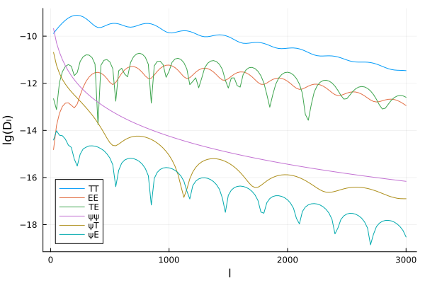
Two-point correlation function
SymBoltz.correlation_function — Function
correlation_function(sol::CosmologySolution; N = 2048, spline = true)Compute the two-point correlation function in real space by Fourier transforming the matter power spectrum of sol with N points the FFTLog algorithm implemented in TwoFAST. Returns N radii and correlation function values (e.g. r, ξ).
Example
using SymBoltz, Plots
M = ΛCDM()
pars = parameters_Planck18(M)
prob = CosmologyProblem(M, pars)
ks = 10 .^ range(-2, +6, length=300)
sol = solve(prob, ks)
rs, ξs = correlation_function(sol)
rs = rs * L100 # convert from c/H₀ to Mpc/h
plot(rs, @. ξs * rs^2; xlims = (0, 200), xlabel = "r / (Mpc/h)", ylabel = "r² ξ / (Mpc/h)²")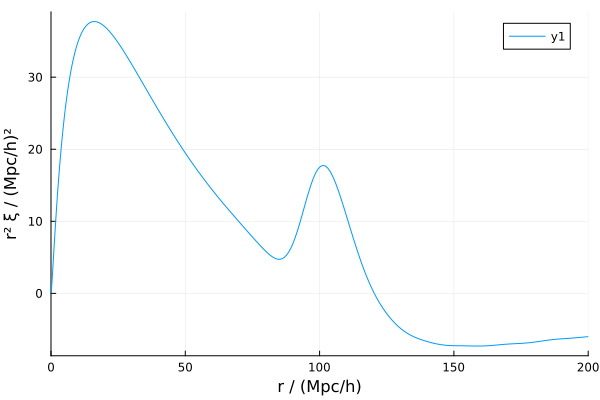
Matter density fluctuations
SymBoltz.variance_matter — Function
variance_matter(sol::CosmologySolution, R)Compute the variance $⟨δ²⟩$ of the linear matter density field with a top-hat filter with radius R in units of $c/H₀$. Wraps the implementation in MatterPower.jl.
SymBoltz.stddev_matter — Function
stddev_matter(sol::CosmologySolution, R)Compute the standard deviation $√(⟨δ²⟩)$ of the linear matter density field with a top-hat filter with radius R in units of $c/H₀$.
using SymBoltz, Plots
M = ΛCDM()
pars = parameters_Planck18(M)
prob = CosmologyProblem(M, pars)
ks = 10 .^ range(-2, +6, length=300)
sol = solve(prob, ks)

Rs = 10 .^ range(0.5, 2.5, length=100) # Mpc/h
σs = stddev_matter.(sol, Rs / L100) # Mpc/h to c/H₀
plot(log10.(Rs), log10.(σs); xlabel = "lg(R / (Mpc/h))", ylabel = "lg(σ)", label = nothing)

σ8 = stddev_matter(sol, 8 / L100) # 8 Mpc/h to c/H₀
scatter!((log10(8), log10(σ8)), series_annotation = text("  σ₈ = $(round(σ8; digits=3))", :left), label = nothing)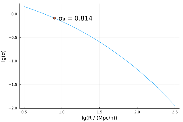
Distance measures
SymBoltz.distance — Function
distance(modes, sol::CosmologySolution, t)Get the distances modes at the values t of the independent variable from the solution sol. The times t can be a vector of values of the independent variable, or a pair like M.g.z => zs with values of another variable. The modes can be one or a vector of:
:χ: line-of-sight comoving distance $χ = τ₀ - τ$,:M: transverse comoving distance $D_M = \sin(\sqrt{-Ω_{k0}} χ) / \sqrt{-Ω_{k0}}$,:A: angular diameter distance $D_A = a D_M$,:L: luminosity distance $D_L = D_M / a$,:H: Hubble distance $D_H = 1 / H$,:V: volume-averaged distance $D_V = (z D_M^2 D_H)^{1/3}$.
Returned distances are dimensionless in units of $c/H₀$. The model must have the variables χ, a and H.
using SymBoltz, Plots
M = ΛCDM()
pars = parameters_Planck18(M)
prob = CosmologyProblem(M, pars)
sol = solve(prob)

τ0 = today(sol)
τs = range(0.5*τ0, τ0, length = 100) # conformal times back in time
zs = sol(M.g.z, τs) # corresponding redshifts
modes = [:χ, :M, :A, :L, :V] # distances from today
Ds = distance(modes, sol, τs)
labels = ["Dχ (lookback distance)" "DM (transverse comoving distance)" "DA (angular diameter distance)" "DL (luminosity distance)" "DV (volume-averaged distance)"]
plot(zs, transpose(Ds); xlabel = "z", ylabel = "D / (c/H₀)", label = labels, xlims = extrema(zs), ylims = (0, 3))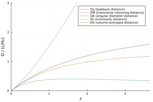
Sound horizon (BAO scale)
SymBoltz.sound_horizon — Function
sound_horizon(sol::CosmologySolution[, t])Get the photon-baryon sound horizon
\[ rₛ(τ) = ∫_0^τ dτ cₛ = ∫_0^τ \frac{dτ}{√(3(1+3ρ_b/4ρ_γ))}\]
at the time steps of the solution sol, or at the values t of the independent variable. It is integrated with the background as the variable rₛ.
SymBoltz.time_drag — Function
time_drag(sol::CosmologySolution)Get the value of the independent time variable $t$ at the baryon drag epoch, when the drag optical depth satisfies
\[ κ_d(t) = -∫_t^{t_0} \frac{κ'}{3ρ_b/4ρ_γ} dt' = 1,\]
where $κ$ is the Thomson optical depth and $κ' = dκ/dt$. The sound horizon at the drag epoch $r_d$ is then sound_horizon(sol, time_drag(sol)).
The BAO scale is the sound horizon at the baryon drag epoch:
using SymBoltz, Plots
M = ΛCDM()
pars = parameters_Planck18(M)
prob = CosmologyProblem(M, pars)
sol = solve(prob)

Mpc = L100 / pars[M.g.h] # (c/H₀) in Mpc
as = sol[M.g.a]
rs = sound_horizon(sol) * Mpc
κd = sol[M.κd]
τd = time_drag(sol)
ad = sol(M.g.a, τd)
zd = sol(M.g.z, τd)
rd = sound_horizon(sol, τd) * Mpc

p = plot(as, rs; xlabel = "a", ylabel = "rs / Mpc", label = "rs(a)", color = 1, xscale = :log10, xlims = (1e-5, 1), ylims = (0, 1300), legend = (0.12, 0.25))
scatter!(p, [ad], [rd]; label = "rs(ad) = $(round(rd; digits = 1)) Mpc", color = 1)
p2 = twinx(p) # right axis
plot!(p2, as[κd .> 0], κd[κd .> 0]; ylabel = "κd", label = "κd(a)", color = 2, yscale = :log10, ylims = (1e-3, 1e3), xscale = :log10, xlims = (1e-5, 1), legend = (0.12, 0.9))
hline!(p2, [1]; color = 2, linestyle = :dash, label = nothing)
scatter!(p2, [ad], [1]; label = "κd(ad) = 1", color = 2)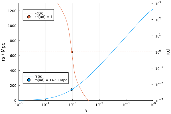
Source functions
SymBoltz.source_grid — Function
source_grid(
    prob::CosmologyProblem, Ss, τs, ks[, bgsols];
    bgalg = default_bgalg(prob), bgreltol = 1e-7, bgabstol = 1e-7, bgopts = (),
    ptalg = default_ptalg(prob), ptreltol = 1e-5, ptabstol = 1e-5, ptopts = (),
    thread = true, verbose = false
)
Compute and evaluate source functions $S(τ,k)$ with symbolic expressions Ss on a grid with conformal times τs and wavenumbers ks from the problem prob. Returns a matrix of size (Nτ, Nk), where each element is a vector of length NS = length(Ss) holding all source values at that (τ, k) point.
The algorithms bgalg/ptalg, tolerances bgreltol/ptreltol and bgabstol/ptabstol and extra options bgopts/ptopts are passed to the background/perturbation ODE solves. If the background solutions bgsols are passed, they are used directly and the background options are not accepted.
using SymBoltz, Plots, DataInterpolations
M = ΛCDM(h = nothing, ν = nothing)
pars = parameters_Planck18(M)
prob = CosmologyProblem(M, pars)
sol = solve(prob)

τs = sol[M.τ] # conformal times in background solution
ks = exp.(range(log(1.0), log(2000.0), length = 50)) # logarithmic k-grid
Ss = source_grid(prob, M.ST, τs, ks)
iτ = argmax(sol[M.b.v]) # index of decoupling time
iτs = iτ-75:iτ+75 # indices around decoupling
p1 = surface(ks, τs[iτs], Ss[iτs, :]; camera = (45, 25), xlabel = "k", ylabel = "τ", zlabel = "S", colorbar = false)

lgas = -6.0:0.2:0.0
τs = LinearInterpolation(sol[M.τ], sol[log10(M.g.a)])(lgas) # τ at given lg(a)
ks = 5.0:5.0:100.0
Ss = source_grid(prob, M.g.Ψ, τs, ks)
p2 = wireframe(ks, lgas, Ss; camera = (75, 20), xlabel = "k", ylabel = "lg(a)", zlabel = "Φ")

plot(p1, p2)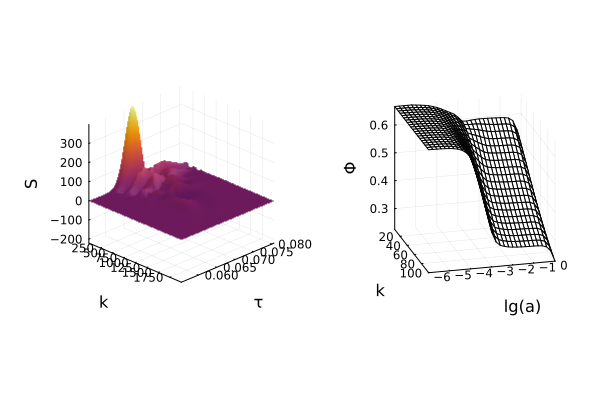
Line-of-sight integration
SymBoltz.los_integrate — Function
los_integrate(Ss::AbstractMatrix{T}, ls::AbstractVector, χs::AbstractVector, ks::AbstractVector, jl::SphericalBesselCache, ws::AbstractVector; l_limber = typemax(Int), thread = true, verbose = false) where {T}For the given ls and ks, compute the line-of-sight integrals
\[Iₗ(k) = ∫dχ S(χ,k) jₗ(kχ)\]
over the source function values Ss against the spherical Bessel functions $jₗ(x)$ cached in jl, using the quadrature weights ws for the descending conformal distances $χ = τ₀ - τ$. The element Ss[i,j] holds the source function value $S(χᵢ, kⱼ)$. The Limber approximation
\[Iₗ ≈ √(π/(2l+1)) S((l+1/2)/k, k)\]
is used for l ≥ l_limber. Contributions where $|jₗ(x)|$ is below jltol (at small $x ≪ l$) are skipped.